Two Carhops Drive-in Queue
2025 — A simulation of which carhop should take the next car at a drive-in
01 Problem
A drive-in restaurant has two carhops, Ali and Badu, who walk out to each car to take its order. Ali is the faster of the two. When a car pulls in and both of them are free, someone has to decide who goes.
The goal is to compare three rules for that moment, picking at random, always sending Ali, or always sending Badu, by how long cars wait and how long each carhop stands idle.
02 Cars
A new car pulls in a gap of 1 to 4 minutes after the last one, most often 2 minutes, so a car arrives every 2.25 minutes on average, a rate of 0.444 cars a minute.
probs_interarrival <- c(0.25, 0.40, 0.20, 0.15)

interarrival <- sample(1:4, n, replace = TRUE, prob = probs_interarrival)
arrival_time <- cumsum(interarrival)
03 Carhops
Ali takes 2 to 5 minutes to serve a car, 3.29 on average. Badu takes 3 to 6 minutes, 4.25 on average.
Neither could keep up with a car every 2.25 minutes alone. With order times and , each minute would bring Ali minutes of orders, or Badu minutes, and both are more than one, so the line would grow without end. Together they finish up to cars a minute, so the load is 82% of what they can handle.
Both are needed, and the rule only matters in the moments when both happen to be free.
probs_ali <- c(0.30, 0.28, 0.25, 0.17); times_ali <- c(2,3,4,5)
probs_badu <- c(0.35, 0.25, 0.20, 0.20); times_badu <- c(3,4,5,6)

sd <- if (server == 1) sample(times_ali, 1, prob = probs_ali) else sample(times_badu, 1, prob = probs_badu)
04 Simulation
Cars are served in the order they arrive. A car that finds one carhop free goes to that one, a car that finds both free goes to whoever the rule picks, and a car that finds both busy waits for whoever finishes first.
The original app runs one evening per random seed. Here each evening is 32 cars, the app's default, repeated for seeds 1 to 20,000 under each rule, so every rule sees the same cars at the same times.
for (i in 1:n) {
  t_arr <- arrival_time[i]
  free_now <- which(next_free <= t_arr)

  if (length(free_now) > 0) {
    if (all(c(1,2) %in% free_now)) {
      if (idle_choice_rule == "random") {
        server <- sample(c(1,2), 1)
      } else if (idle_choice_rule == "ali") {
        server <- 1
      } else {
        server <- 2
      }
    } else {
      server <- free_now[1]
    }
    start <- t_arr
  } else {
    server <- which.min(next_free)
    start <- next_free[server]
  }

  finish <- start + sd
  next_free[server] <- finish
}

waiting_time <- start_service_time - arrival_time
05 Exact wait
The simulation only estimates the wait, but the model is small enough to solve exactly. A new car only needs to know how many minutes of work Ali and Badu have left when it pulls in, and for car . It waits for whoever finishes first, so its wait is the smaller of the two, which is zero when either is free.
The car goes to whoever has less left. On a tie the rule picks if both are free, and Ali goes if both are busy, because the app's which.min takes the first carhop. The chosen carhop's work grows by one order time, the next car comes a gap later, and both counts drop by but never below zero.
The next pair depends only on the current one, so the pairs form a Markov chain. Every evening starts with an empty lot, , and the chance of each pair is the sum over every pair, choice , order time , and gap that leads to it. The choice is certain, except that a random pick gives each carhop half when both are free.
Weighting each pair's wait by its chance gives the expected wait of each car, and averaging over cars gives the exact average wait of an -car evening. The first two cars never wait, since the first finds both carhops free and the second finds the one who did not take the first.
06 Answer
Across 20,000 evenings, cars wait 40.0 s on average when Ali goes first, 41.2 s with a random pick, and 42.3 s when Badu goes first. Sending the faster carhop saves about 2.3 s a car.
Following the chain car by car gives the exact average wait for 32 cars. It is 40.2 s with Ali first, 41.4 s with a random pick, and 42.5 s with Badu first. Waits grow as the queue builds from an empty lot, reaching 48.8 s with Ali first over 128 cars, and Ali first never does worse at any evening length.
07 One evening
The gap is small next to the swing of a single evening. The average wait of one 32-car evening has a standard deviation of 37.3 s, about 16 times the gap between Ali first and Badu first.
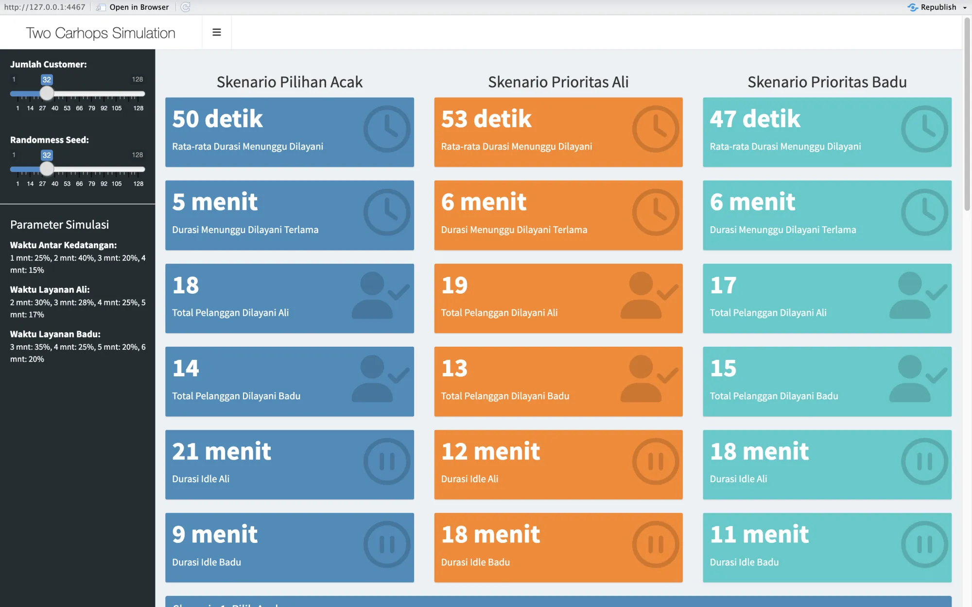
The original app opens on seed 32, where Badu first looks best at 47 seconds against 50 for a random pick and 53 for Ali first. Across all 128 of the app's seeds, Ali first gives the shorter wait in 66, Badu first gives it in 32, and they tie in 30.
sim_random <- reactive({ run_simulation(input$n_customer, "random", input$seed_value) })
sim_to_ali <- reactive({ run_simulation(input$n_customer, "ali", input$seed_value) })
sim_to_badu <- reactive({ run_simulation(input$n_customer, "badu", input$seed_value) })
08 Workload
The rule also decides who does the work. With Ali first, Ali serves 19.7 of the 32 cars and stands idle for 10.9 min, while Badu stands idle for 22.7 min. Badu first nearly evens out the cars at 16.5 to 15.5, and leaves Ali idle for 20.9 min.
A random pick sits in between and splits the idle time most evenly, at 16.3 min for Ali and 15.9 min for Badu.
idle_time_srv[server] <- idle_time_srv[server] + max(0, start - last_finish[server])

busy_time[server] <- busy_time[server] + sd
last_finish[server] <- finish
09 Original app
The simulation was first built in R as an interactive Shiny dashboard. Two sliders set the number of cars and the random seed, each from 1 to 128, and the three rules sit side by side with their average and longest wait, cars served, and idle time for each carhop, above a table of every car under each rule.
It is still live on shinyapps.io. The free tier puts the app to sleep when nobody is using it, so the first visit can take a while to load.
10 Limits
The original app stops each carhop's idle clock at their own last order, so time spent idle while the other carhop finishes the last cars is not counted. Counting until the last car leaves adds up to two minutes per carhop, raising Badu's idle time under Ali first from 22.7 min to 24.4 min, but leaves the comparison between rules the same.
Every evening starts with an empty lot, so short evenings understate the wait a busy lot settles into. The times are whole minutes and the probabilities are assumptions, not measurements from a real drive-in, and no car ever gives up and leaves. Timed orders from a real lot would make the answer worth trusting.
Two Carhops Drive-in Queue
Sending Ali first cuts the wait to 40.0 s a car over 20,000 simulated evenings